The `ikeogu.2017` data set contains raw vis-NIRS scans, total carotenoid content, and cassava root dry matter content (using the oven method) from the 2017 PLOS One paper by Ikeogu et al. This dataset contains a subset of the original scans and reference values from the supplementary files of the paper. `ikeogu.2017` is a `data.frame` that contains the following columns:
study.name = Name of the study as described in Ikeogu et al. (2017).
sample.id = Unique identifier for each individual root sample
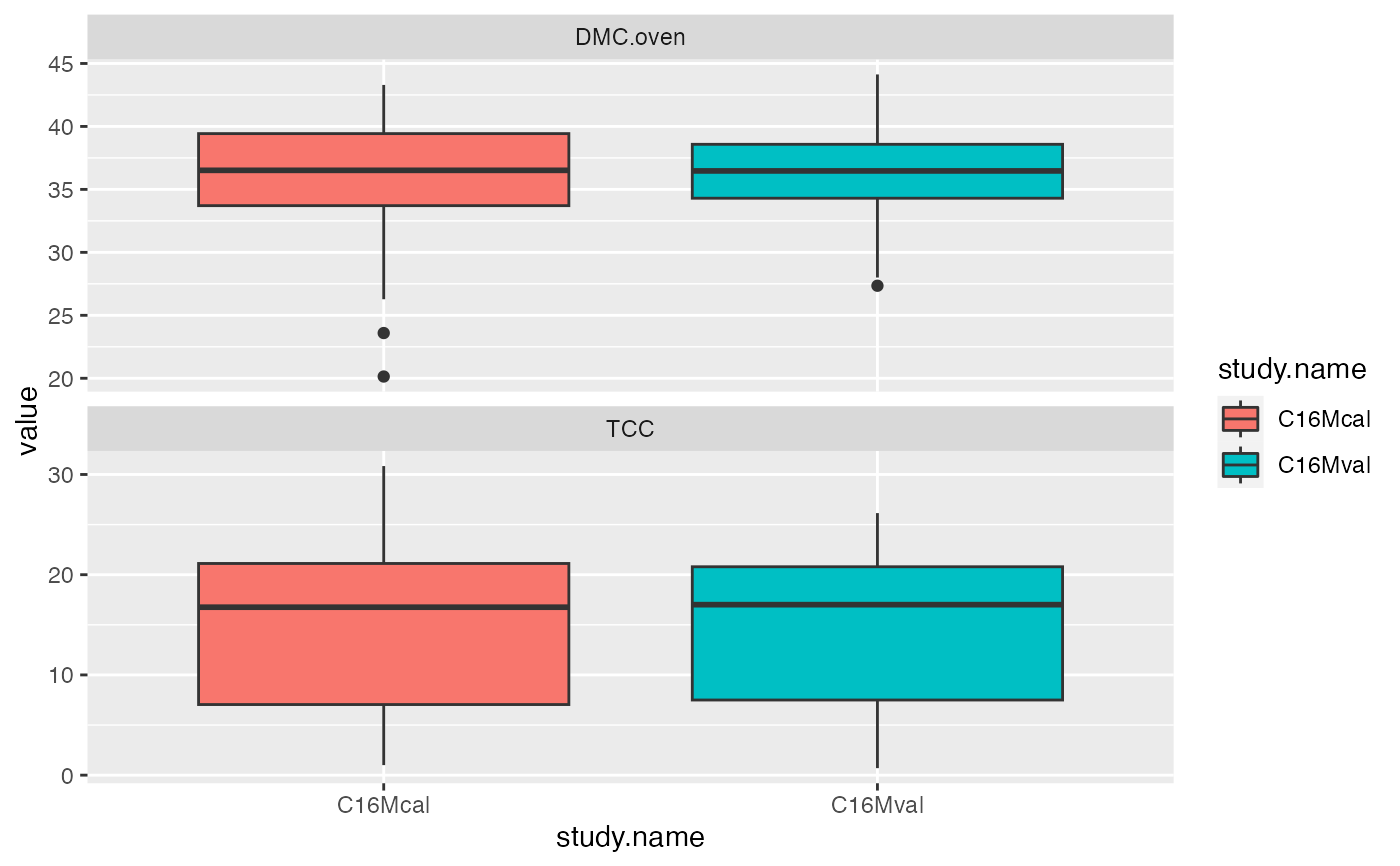
DMC.oven = Cassava root dry matter content, the percentage of dry weight relative to fresh weight of a sample after oven drying.
TCC = Total carotenoid content (\(\mu g/g\), unknown whether on a fresh or dry weight basis) as measured by high performance liquid chromatography
X350:X2500 = spectral reflectance measured with the QualitySpec Trek: S-10016 vis-NIR spectrometer. Each cell represents the mean of 150 scans on a single root at a single wavelength.
References
Ikeogu, U.N., F. Davrieux, D. Dufour, H. Ceballos, C.N. Egesi, et al. 2017. Rapid analyses of dry matter content and carotenoids in fresh cassava roots using a portable visible and near infrared spectrometer (Vis/NIRS). PLOS One 12(12): 1–17. doi: 10.1371/journal.pone.0188918.
Author
Original authors: Ikeogu, U.N., F. Davrieux, D. Dufour, H. Ceballos, C.N. Egesi, and J. Jannink. Reformatted by Jenna Hershberger.
Examples
library(magrittr)
library(ggplot2)
data(ikeogu.2017)
ikeogu.2017[1:10, 1:10]
#> # A tibble: 10 × 10
#>    study.name sample.id  DMC.oven   TCC  X350  X351  X352  X353  X354  X355
#>    <chr>      <chr>         <dbl> <dbl> <dbl> <dbl> <dbl> <dbl> <dbl> <dbl>
#>  1 C16Mcal    C16Mcal_1      39.6  1.00 0.488 0.495 0.506 0.494 0.500 0.496
#>  2 C16Mcal    C16Mcal_2      35.5 17.0  0.573 0.568 0.599 0.593 0.581 0.597
#>  3 C16Mcal    C16Mcal_3      42.0 21.6  0.599 0.627 0.624 0.606 0.607 0.624
#>  4 C16Mcal    C16Mcal_4      39.0  2.43 0.517 0.516 0.514 0.536 0.542 0.536
#>  5 C16Mcal    C16Mcal_5      33.4 24.0  0.519 0.548 0.554 0.549 0.549 0.567
#>  6 C16Mcal    C16Mcal_6      32.1 19.0  0.576 0.566 0.589 0.591 0.613 0.628
#>  7 C16Mcal    C16Mcal_7      35.8  6.61 0.530 0.536 0.525 0.539 0.537 0.529
#>  8 C16Mcal    C16Mcal_8      26.3 14.1  0.596 0.596 0.602 0.608 0.604 0.610
#>  9 C16Mcal    C16Mcal_9      38.1 28.9  0.675 0.662 0.688 0.694 0.697 0.695
#> 10 C16Mcal    C16Mcal_10     31.8 18.4  0.510 0.527 0.535 0.538 0.542 0.551
ikeogu.2017 %>%
  dplyr::select(-starts_with("X")) %>%
  dplyr::group_by(study.name) %>%
  tidyr::pivot_longer(cols = c(DMC.oven:TCC), names_to = "trait", values_to = "value") %>%
  tidyr::drop_na(value) %>%
  ggplot2::ggplot(aes(x = study.name, y = value, fill = study.name)) +
  facet_wrap(~trait, scales = "free_y", nrow = 2) +
  geom_boxplot()