waves

library(waves)
library(magrittr)
library(dplyr)
library(tidyr)
library(ggplot2)
library(tibble)

Introduction

Originally designed application in the context of resource-limited plant research and breeding programs, waves provides an open-source solution to spectral data processing and model development by bringing useful packages together into a streamlined pipeline. This package is wrapper for functions related to the analysis of point visible and near-infrared reflectance measurements. It includes visualization, filtering, aggregation, pretreatment, cross-validation set formation, model training, and prediction functions to enable open-source association of spectral and reference data.

Use

Follow the installation instructions below, and then go wild! Use waves to analyze your own data. Please report any bugs or feature requests by opening issues in the waves repository.

Installation

Install the latest waves release directly from CRAN:

install.packages("waves")
library(waves)

Alternatively, install the development version to get the most up-to-date (but not necessarily thoroughly tested) version:

install.packages("devtools")
devtools::install_github("GoreLab/waves")
library(waves)

1. Format your data

Match spectra with reference values so that you have a data.frame with unique identifiers, reference values, and other metadata as columns to the left of spectral values. Spectral column names should start with “X”. Remove rows with missing values.

ikeogu.2017[1:7, 1:7]
#> # A tibble: 7 × 7
#>   study.name sample.id DMC.oven   TCC  X350  X351  X352
#>   <chr>      <chr>        <dbl> <dbl> <dbl> <dbl> <dbl>
#> 1 C16Mcal    C16Mcal_1     39.6  1.00 0.488 0.495 0.506
#> 2 C16Mcal    C16Mcal_2     35.5 17.0  0.573 0.568 0.599
#> 3 C16Mcal    C16Mcal_3     42.0 21.6  0.599 0.627 0.624
#> 4 C16Mcal    C16Mcal_4     39.0  2.43 0.517 0.516 0.514
#> 5 C16Mcal    C16Mcal_5     33.4 24.0  0.519 0.548 0.554
#> 6 C16Mcal    C16Mcal_6     32.1 19.0  0.576 0.566 0.589
#> 7 C16Mcal    C16Mcal_7     35.8  6.61 0.530 0.536 0.525

ikeogu.2017.prepped <- ikeogu.2017 %>%
  dplyr::rename(unique.id = sample.id,
                reference = DMC.oven) %>%
  dplyr::select(unique.id, dplyr::everything(), -TCC) %>%
  na.omit()

ikeogu.2017.prepped[1:7, 1:7]
#> # A tibble: 7 × 7
#>   unique.id study.name reference  X350  X351  X352  X353
#>   <chr>     <chr>          <dbl> <dbl> <dbl> <dbl> <dbl>
#> 1 C16Mcal_1 C16Mcal         39.6 0.488 0.495 0.506 0.494
#> 2 C16Mcal_2 C16Mcal         35.5 0.573 0.568 0.599 0.593
#> 3 C16Mcal_3 C16Mcal         42.0 0.599 0.627 0.624 0.606
#> 4 C16Mcal_4 C16Mcal         39.0 0.517 0.516 0.514 0.536
#> 5 C16Mcal_5 C16Mcal         33.4 0.519 0.548 0.554 0.549
#> 6 C16Mcal_6 C16Mcal         32.1 0.576 0.566 0.589 0.591
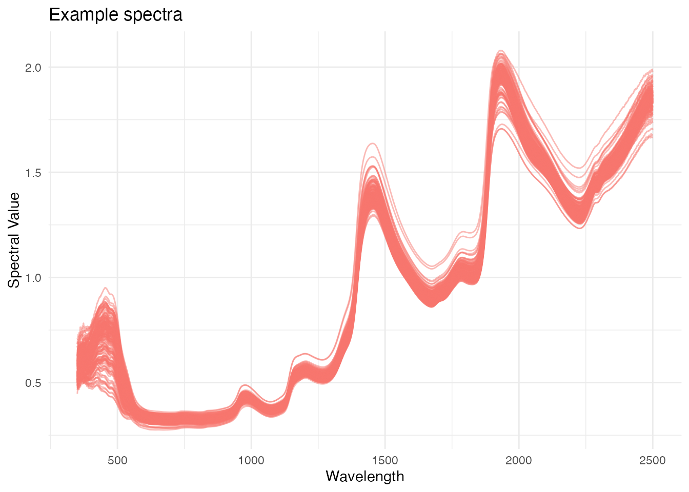
#> 7 C16Mcal_7 C16Mcal         35.8 0.530 0.536 0.525 0.539

2. Visualize spectra with `plot_spectra()`

To display outliers in a different color, set detect.outliers to TRUE.

ikeogu.2017.prepped %>%
  plot_spectra(
    df = .,
    num.col.before.spectra = 5,
    detect.outliers = FALSE,
    alternate.title = "Example spectra"
  )

3. Perform outlier removal with `filter_spectra()`.

waves uses Mahalanobis distance to identify outliers. Mahalanobis distance is a common metric used to identify multivariate outliers. The larger the value of Mahalanobis distance, the more unusual the data point (i.e., the more likely it is to be a multivariate outlier).

The distance tells us how far an observation is from the center of the cloud, taking into account the shape (covariance) of the cloud as well.

To detect outliers, the calculated Mahalanobis distance is compared against a $\chi^2$ distribution with degrees of freedom equal to the number of spectral data columns and an alpha level of 0.05.

filtered.df <- ikeogu.2017.prepped %>%
  filter_spectra(
    df = .,
    filter = TRUE,
    return.distances = TRUE,
    num.col.before.spectra = 5,
    window.size = 15
    )
#> 
#> Removed 0 rows.

filtered.df[1:5, c(1:5, (ncol(filtered.df) - 3):ncol(filtered.df))]
#>   unique.id study.name reference      X350      X351    X2497    X2498    X2499
#> 1 C16Mcal_1    C16Mcal  39.62109 0.4881079 0.4951843 1.866739 1.867465 1.870405
#> 2 C16Mcal_2    C16Mcal  35.52017 0.5727389 0.5682541 1.893840 1.901451 1.891114
#> 3 C16Mcal_3    C16Mcal  42.04462 0.5989934 0.6266454 1.834644 1.828793 1.826562
#> 4 C16Mcal_4    C16Mcal  39.00999 0.5169374 0.5164186 1.837023 1.836635 1.835856
#> 5 C16Mcal_5    C16Mcal  33.44273 0.5189608 0.5477946 1.900873 1.897076 1.899430
#>      X2500
#> 1 1.870702
#> 2 1.888507
#> 3 1.832022
#> 4 1.834857
#> 5 1.896130

No outliers were identified in the example dataset. Note the if return.distances is set to TRUE, the rightmost column contains Mahalanobis distances (h.distances).

4. Aggregate scans

If you have more than one scan per unique identifier, aggregate the scans by mean or median with aggregate_spectra().

In this example, we will aggregate by study.name.

aggregated.test <- ikeogu.2017.prepped %>%
  aggregate_spectra(
    grouping.colnames = c("study.name"),
    reference.value.colname = "reference",
    agg.function = "mean"
    )
aggregated.test[, 1:5]
#> # A tibble: 2 × 5
#>   study.name reference  X350  X351  X352
#>   <chr>          <dbl> <dbl> <dbl> <dbl>
#> 1 C16Mcal         36.1 0.559 0.562 0.569
#> 2 C16Mval         36.4 0.545 0.549 0.552

5. Evaluate the predictive ability of your spectra

test_spectra() is a wrapper that performs spectral pretreatment (5.1), cross-validation set formation (5.2), and model training functions over multiple iterations (5.3).

Note that the following subsections describe functions that are called within test_spectra(). They do not need to be used separately for model pretreatment, cross-validation set formation, or model training.

Some of the arguments for this function are detailed below. A description of output is below under section 5.4. See ?test_spectra() for more information on the arguments and output for this function.

results.list <- ikeogu.2017.prepped %>%
  dplyr::select(unique.id, reference, dplyr::starts_with("X")) %>%
  na.omit() %>%
  test_spectra(
    train.data = .,
    tune.length = 3,
    num.iterations = 3,
    pretreatment = 1
    )
#> Pretreatment initiated.
#> Training models...
#> Working on Raw_data
#> Returning model...

5.1. Pretreat spectra

Specify which spectral pretreatments (1-13) to apply with the parameter pretreatment. pretreat_spectra() can also be used on its own to transform a data.frame using any/all of 12 available pretreatments:

Raw data (no pretreatment is applied)
Standard normal variate (SNV)
SNV and first derivative
SNV and second derivative
First derivative
Second derivative
Savitzky–Golay filter (SG)
SNV and SG
Gap segment derivative (window size = 11)
SG and first derivative (window size = 5)
SG and first derivative (window size = 11)
SG and second derivative (window size = 5)
SG and second derivative (window size = 11)

ikeogu.2017.prepped[1:10, ] %>% # subset the first 10 scans for speed
  pretreat_spectra(pretreatment = 2:13) %>% # exclude pretreatment 1 (raw data)
  bind_rows(.id = "pretreatment") %>%
  gather(key = "wl",
         value = "s.value",
         tidyselect::starts_with("X")) %>%
  mutate(wl = as.numeric(readr::parse_number(.data$wl)),
         pretreatment = as.factor(pretreatment)) %>%
  drop_na(s.value) %>%
  ggplot(data = ., aes(x = wl, y = s.value, group = unique.id)) +
  geom_line(alpha = .5) +
  theme(axis.text.x = element_text(angle = 45)) +
  labs(title = "Pretreated spectra",
       x = "Wavelength",
       y = "Spectral Value") +
  facet_wrap(~ pretreatment, scales = "free")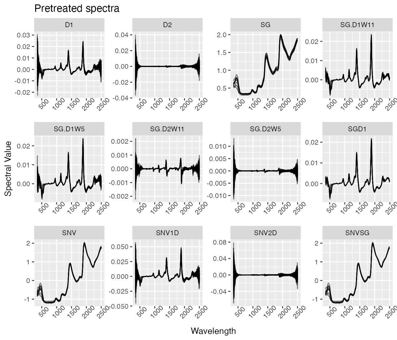

Note that the scales in this plot are “free”. Without free scales, anything derivative-based treatment (D1 or D2) looks like it’s a constant zero in comparison to those without derivative-based treatments (SNV, SG).

5.2. Specify a cross-validation scheme

Choose from random, stratified random, or a plant breeding-specific scheme from Jarquín et al., 2017. The Plant Genome. Options include:

`cv.scheme`	Description
`NULL`	Random or stratified random sampling (does not take genotype or environment into account)
“CV1”	Untested lines in tested environments
“CV2”	Tested lines in tested environments
“CV0”	Tested lines in untested environments
“CV00”	Untested lines in untested environments

If cv.scheme is set to NULL, the argument stratified.sampling is used to determine whether stratified random sampling should be performed. If TRUE, the reference values from the input data.frame (train.data) will be used to create a balanced split of data between the training and test sets in each training iteration.

When using one of the four specialized cross-validation schemes (“CV1”, “CV2”, “CV0”, or “CV00”), additional arguments are required: - trial1 contains the trial to be tested in subsequent model training functions. The first column contains unique identifiers, second contains genotypes, third contains reference values, followed by spectral columns. Include no other columns to right of spectra! Column names of spectra must start with “X”, reference column must be named “reference”, and genotype column must be named “genotype”. -trial2 contains a trial that has overlapping genotypes with trial1 but that were grown in a different site/year (different environment). Formatting must be consistent with trial1. - trial3 contains a trial that may or may not contain genotypes that overlap with trial1. Formatting must be consistent with trial1.

Cross-validation schemes can also be formatted outside of test_spectra() using the function format_cv().

5.3. Train spectral prediction models

Many of the arguments for test_spectra() are related to model training: - model.method is the algorithm type to use for training. See the table below for more information - tune.length is the number of PLS components to test. This argument is ignored if other algorithms are used - best.model.metric indicates the metric used to decide which model is best (“RMSE” or “R-squared”) - k-fold specifies the number of folds used for cross-validation to tune model hyperparameters within the training set - num.iterations sets the number of training iterations - proportion.train is the fraction of samples to be included in the training set (default is 0.7)

Models can also be trained with the standalone function train_spectra(). Model training is implemented with caret.

Algorithm	`model.method`	R package source	Tuning parameters (hyperparameters)
Partial least squares (PLS)	“pls”	`pls`	ncomp
Random forest (RF)	“rf”	`randomForest`	mtry
Support vector machine (SVM) with linear kernel	“svmLinear”	`kernlab`	C
Support vector machine (SVM) with radial kernel	“svmRadial	`kernlab`	sigma, C

5.4. Output

test_spectra() outputs a list with four objects:

model.list is a list of trained model objects, one for each pretreatment method specified by the pretreatment argument. Each model is trained with all rows of the input data.frame (df)

summary(results.list$model)
#> Data:    X dimension: 173 2151 
#>  Y dimension: 173 1
#> Fit method: kernelpls
#> Number of components considered: 3
#> TRAINING: % variance explained
#>            1 comps  2 comps  3 comps
#> X            62.65    68.38    91.17
#> reference    63.34    75.71    76.87

summary.model.performance is a data.frame containing summary statistics across all model training iterations and pretreatments. See below for a description of the summary statistics provided.

results.list$summary.model.performance
#>   SummaryType ModelType     RMSEp        R2p      RPD      RPIQ        CCC
#> 1        mean       pls 2.0440540 0.77824381 2.085018 2.6038009 0.85155095
#> 2          sd       pls 0.2661027 0.02093217 0.183391 0.3062501 0.04696515
#> 3        mode       pls 1.8971232 0.78270780 2.139263 2.7700624 0.86628031
#>          Bias       SEP     RMSEcv      R2cv       R2sp best.ncomp best.ntree
#> 1 -0.05516781 2.0652364 1.95463427 0.7755627 0.77670789          3         NA
#> 2  0.09468830 0.2688604 0.08412512 0.0157923 0.01211986          0         NA
#> 3 -0.13588174 1.9167831 1.96423744 0.7807426 0.76866372          3         NA
#>   best.mtry
#> 1        NA
#> 2        NA
#> 3        NA

model.performance is a data.frame containing performance statistics for each iteration of model training separately (see below).

results.list$model.performance
#>   Iteration ModelType    RMSEp       R2p      RPD     RPIQ       CCC
#> 1         1       pls 1.897123 0.7827078 2.139263 2.770062 0.8662803
#> 2         2       pls 1.883812 0.7965839 2.235167 2.790961 0.8893859
#> 3         3       pls 2.351227 0.7554397 1.880623 2.250380 0.7989866
#>          Bias      SEP   RMSEcv      R2cv      R2sp best.ncomp best.ntree
#> 1 -0.13588174 1.916783 1.964237 0.7807426 0.7686637          3         NA
#> 2  0.04906262 1.903334 2.033546 0.7578310 0.7708123          3         NA
#> 3 -0.07868431 2.375593 1.866120 0.7881145 0.7906476          3         NA
#>   best.mtry
#> 1        NA
#> 2        NA
#> 3        NA

predictions is a data.frame containing both reference and predicted values for each test set entry in each iteration of model training.

head(results.list$predictions)
#>   Iteration ModelType  unique.id reference predicted
#> 1         1       pls  C16Mcal_3  42.04462  39.73413
#> 2         1       pls C16Mcal_11  35.23000  37.05843
#> 3         1       pls C16Mcal_14  42.23797  41.23787
#> 4         1       pls C16Mcal_16  36.37963  38.47196
#> 5         1       pls C16Mcal_17  36.62819  38.38934
#> 6         1       pls C16Mcal_21  37.61227  37.58763

importance is a data.frame containing variable importance results for each wavelength at each iteration of model training. If model.method is not “pls” or “rf”, this list item is NULL.

results.list$importance[, 1:7]
#> # A tibble: 3 × 7
#>   Iteration ModelType   X350   X351   X352   X353   X354
#>       <int> <chr>      <dbl>  <dbl>  <dbl>  <dbl>  <dbl>
#> 1         1 pls       0.0258 0.0245 0.0278 0.0268 0.0265
#> 2         2 pls       0.0351 0.0344 0.0329 0.0315 0.0328
#> 3         3 pls       0.0241 0.0251 0.0256 0.0258 0.0253

Statistic*	Description
RMSE_p	Root mean squared error of prediction
R²_p	Squared Pearson’s correlation between predicted and observed test set values
RPD	Ratio of standard deviation of observed test set values to RMSE_p
RPIQ	Ratio of performance to interquartile difference
CCC	Concordance correlation coefficient
Bias	Average difference between the predicted and observed values
SEP	Standard error of prediction
RMSE_cv	Root mean squared error of cross-validation
R²_cv	Coefficient of multiple determination of cross-validation for PLS models
R²_sp	Squared Spearman’s rank correlation between predicted and observed test set values
best.ncomp	Best number of components in a PLS model
best.ntree	Best number of trees in an RF model
best.mtry	Best number of variables to include at every decision point in an RF model

*Many of the spectral model performance statistics are calculated using the function postResampleSpectro() from the spectacles package.

6. Save trained prediction models with `save_model()`

Intended for a production environment
Can evaluate spectral pretreatment methods using the input dataset
Selects best model using the metric provided with best.model.metric (“RMSE” or “Rsquared”)
Returns trained model with option to save as .Rds object
The $model output from test_spectra() can also be saved and used for prediction, but save_model() will take the extra step of saving an .Rds file for you if write.model is set to TRUE.

In the example below, we’ll use one subset of the example dataset (“C16Mcal”) to create the model and then we’ll predict the other subset (“C16Mval”) in section 7.

model.to.save <- ikeogu.2017.prepped %>%
  dplyr::filter(study.name == "C16Mcal") %>%
  dplyr::select(unique.id, reference, dplyr::starts_with("X")) %>%
  na.omit() %>%
  save_model(
    df = .,
    write.model = FALSE,
    pretreatment = c(1, 2, 8),  # Raw, SNV, and SNVSG (typically best performers)
    tune.length = 3,
    num.iterations = 2,
    verbose = FALSE
    )

Now let’s take a look at our trained model:

summary(model.to.save$best.model)
#> Data:    X dimension: 120 2141 
#>  Y dimension: 120 1
#> Fit method: kernelpls
#> Number of components considered: 3
#> TRAINING: % variance explained
#>            1 comps  2 comps  3 comps
#> X            64.48    87.94    91.43
#> reference    33.93    64.97    87.18

model.to.save$best.model.stats %>%
  gather(key = "statistic", value = "value", RMSEp_mean:best.mtry_mode) %>%
  separate(statistic, into =  c("statistic", "summary_type"), sep = "_") %>%
  pivot_wider(id_cols = c(Pretreatment, summary_type),
              names_from = statistic, values_from = value)
#> # A tibble: 3 × 15
#>   Pretreatment summary_type RMSEp    R2p   RPD  RPIQ    CCC   Bias   SEP RMSEcv
#>   <chr>        <chr>        <dbl>  <dbl> <dbl> <dbl>  <dbl>  <dbl> <dbl>  <dbl>
#> 1 SNVSG        mean         1.71  0.845  2.55  3.19  0.907  -0.140 1.73  1.57  
#> 2 SNVSG        sd           0.299 0.0572 0.398 0.604 0.0320  0.442 0.303 0.0145
#> 3 SNVSG        mode         1.50  0.885  2.83  3.61  0.930  -0.453 1.52  1.56  
#> # ℹ 5 more variables: R2cv <dbl>, R2sp <dbl>, best.ncomp <dbl>,
#> #   best.ntree <dbl>, best.mtry <dbl>

7. Predict phenotypic values with new spectra

If generating predictions from a saved model file in .Rds format, use predict_spectra(). If the model object is already in your R environment, the function stats::predict() can be used to generate predictions. predict_spectra() pulls the best model hyperparameters from your saved model object, but if using stats::predict(), these must be supplied separately.

Using the model we trained in section 6, we can predict cassava root dry matter content for our held out validation set:

First, determine which pretreatment generated the best model and pretreat the new spectral dataset accordingly.

# Get the best pretreatment number from model stats
best.pretreatment.name <- model.to.save$best.model.stats$Pretreatment
best.pretreatment.num <- match(best.pretreatment.name, 
                               c("Raw_data", "SNV", "SNV1D", "SNV2D", "D1", "D2", "SG",
                                 "SNVSG", "SGD1", "SG.D1W5", "SG.D1W11", "SG.D2W5", "SG.D2W11"))

# Use the example validation set (C16Mval)
pretreated.val <- ikeogu.2017.prepped %>%
  dplyr::filter(study.name == "C16Mval") %>%
  pretreat_spectra(pretreatment = best.pretreatment.num)

pretreated.val.mx <- pretreated.val %>%
  dplyr::select(starts_with("X")) %>%
  as.matrix()

best.ncomp <- model.to.save$best.model.stats$best.ncomp_mode

Perform predictions!

predicted.values <- as.numeric(predict(model.to.save$best.model,
                                       newdata = pretreated.val.mx,
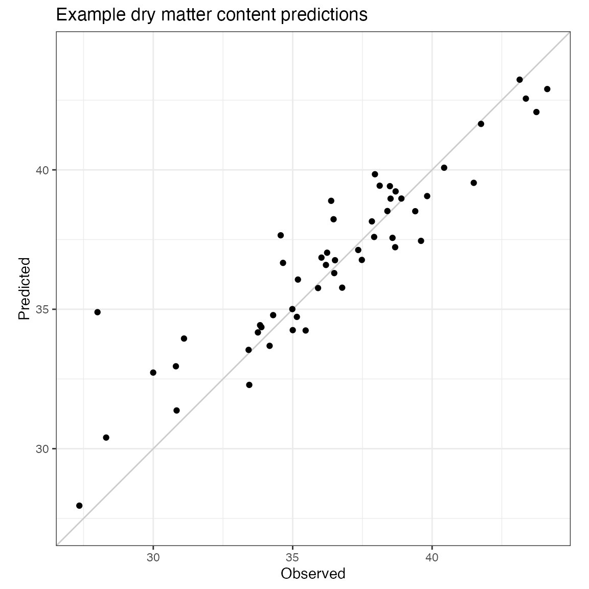
                                       ncomp = best.ncomp))

How did we do?

spectacles::postResampleSpectro(pred = predicted.values,
                                obs = pretreated.val$reference)
#>      RMSE  Rsquared       RPD      RPIQ       CCC      Bias        SE 
#> 1.5560069 0.8420531 2.4672707 2.7511960 0.9009541 0.1604845 1.5708972

Plot predictions

overall.range <- c(min(c(pretreated.val$reference, predicted.values)),
                   max(c(pretreated.val$reference, predicted.values)))
cbind(unique.id = pretreated.val$unique.id,
      observed = pretreated.val$reference,
      predicted = predicted.values) %>%
  as_tibble() %>%
  mutate(observed = as.numeric(observed),
         predicted = as.numeric(predicted)) %>%
  ggplot(aes(x = observed, y = predicted)) +
  geom_abline(intercept = 0,
              slope = 1,
              color = "gray80") +
  geom_point() +
  coord_fixed(xlim = overall.range,
              ylim = overall.range) +
  labs(title = "Example dry matter content predictions",
       x = "Observed",
       y = "Predicted") +
  theme_bw()